Data Analysis - Predicting Kickstarter Campaign Success
Author: John Salisbury / Last Updated: Apr 11, 2023
Author: John Salisbury / Last Updated: Apr 11, 2023
In this project, I clean and analyze data on over 250k Kickstarter crowdfunding campaigns that took place in the United States between 2009-2018, using logistic regression to identify factors that predict campaign success.
In this particular notebook, I run and interpret a logistic regression model, allowing me to determine if certain factors in our dataset can predict whether or not Kickstarter campaigns succeed. To view the exploration and cleaning of this dataset, visit this link (or click on "View Data Exploration/Cleaning" above).
--
Table of Contents:
Import Modules and Data
Pre-Model Checks
Run a Logistic Regression
Model Interpretation
--
Find the data for this project on Kaggle:
Kickstarter Projects
To begin our analysis, we first import a number of common Python modules (e.g., NumPy, Pandas, etc.) to our project. We also import the statsmodels module, which will allow us to run a logistic regression in which we can easily interpret beta coefficients from the final model:
#IMPORT MODULES ------

#Stats modules
import statsmodels.api as sm
from statsmodels.stats.outliers_influence import variance_inflation_factor

#Helper modules
import matplotlib.pyplot as plt   #Plotting support
import numpy as np   #Array support
import pandas as pd   #DataFrame support
import seaborn as sns   #Plotting support

#Suppress warnings in Jupyter
import warnings
warnings.filterwarnings('ignore')

#IPython - HTML notebook formatting
from IPython.core.display import HTML
We'll also add some CSS to improve the look and feel of our notebook:
HTML("""
<style>
.jp-needs-light-background {
    display: block;
    margin: auto;
}

.jp-OutputArea-output.jp-RenderedHTMLCommon table {
    margin: 2em auto;
    background: #eae9e9;
    border: 1px solid #000;
    font-size: 12px;
}

.toc {
    font-size: 16px;
}

.nest-one {
    margin-left: 1em;
    font-style: italic;
    font-size: 14px;
}

.nest-two {
    margin-left: 3em;
    font-style: italic;
    font-size: 12px;
}

.faint {
    opacity: 0.2;
}
</style>
""")
And finally, we import our cleaned data as a dataframe:
#IMPORT DATA ------

#Import CSV as DataFrame
data = pd.read_csv("../data/cleaned_data.csv")
Let's just look at the head of our dataframe to verify that everything looks OK:
data.head()
| Name | Goal | Backers | State | fund_days | name_len | years_since | s_winter | s_spring | s_summer | s_fall | |
|---|---|---|---|---|---|---|---|---|---|---|---|
| 0 | Grace Jones Does Not Give A F$#% T-Shirt (limi... | 1000 | 30 | 0 | 39.123056 | 59 | 0 | 0 | 1 | 0 | 0 |
| 1 | CRYSTAL ANTLERS UNTITLED MOVIE | 80000 | 3 | 0 | 87.994525 | 30 | 0 | 0 | 1 | 0 | 0 |
| 2 | drawing for dollars | 20 | 3 | 1 | 8.088854 | 19 | 0 | 0 | 1 | 0 | 0 |
| 3 | Offline Wikipedia iPhone app | 99 | 25 | 1 | 79.266424 | 28 | 0 | 0 | 1 | 0 | 0 |
| 4 | Pantshirts | 1900 | 10 | 0 | 28.409271 | 10 | 0 | 0 | 1 | 0 | 0 |
Looks good! As a reminder our response variable is State, a categorical variable that represents the outcome of each Kickstarter campaign. State has two levels, 0 for "Failed" and 1 for "Successful". Additionally, we have the following explanatory variables that we may decide to integrate into our logistic regression model:
Goal (fundraising goal; continuous)Backers (number of individuals who donated; continuous)fund_days (duration of campaign in days; continuous)name_len (length of campaign name in characters; discrete)years_since (years since Kickstarter launch in 2009)s_winter (indicates if campaign was launched during winter months; categorical)s_spring (indicates if campaign was launched during spring months; categorical)s_summer (indicates if campaign was launched during summer months; categorical)s_fall (indicates if campaign was launched during fall months; categorical)Let's move on with our analysis below.
The next step in our analysis is to conduct a few pre-model checks and ensure that our data meets some of the basic conditions necessary to use it in a logistic regression model.
The first condition our data needs to meet is that the response variale in our model has a binary outcome. As described in the section above, our response variable is State, which is categorical and has values of 0 (indicating a failed Kickstarter campaign) and 1 (indicating a successful campaign).. Since State has only two possible outcomes, we can confirm that this condition has been met.
The next condition our data needs to meet is that the observations in our dataset are independent of each other. The data in our dataset represents over 250+ unique Kickstarter campaigns from across the United States that were launched at different points between 2009-2018. There are no duplicate records or repeated measurements in our dataset. Additionally, we do not have any type of nested or hierarchical structure in our data that would necessitate a more complex type of model. Thus, we can probably go ahead and assume that the observations in our dataset are independent of each other.
Next, we need to verify that there is no colinearity between our numeric explanatory variables. If colinearity is present, we will need to remove correlated variables until colinearity is no longer an issue. To check for colinearity between our explanatory variables, we can (1) pull these variables into a dataframe and (2) create a correlation matrix that displays correlation coefficients between all possible combinations of these variables:
#Investigate colinearity between potential explanatory variables

#Isolate numeric variables
cols = ["Goal", "Backers", "fund_days", "name_len", "years_since"]
expl = data[cols]

#Create correlation matrix
expl.corr()
| Goal | Backers | fund_days | name_len | years_since | |
|---|---|---|---|---|---|
| Goal | 1.000000 | 0.006245 | 0.020847 | -0.006465 | 0.015745 |
| Backers | 0.006245 | 1.000000 | -0.001251 | 0.020870 | 0.025893 |
| fund_days | 0.020847 | -0.001251 | 1.000000 | 0.017794 | -0.197098 |
| name_len | -0.006465 | 0.020870 | 0.017794 | 1.000000 | -0.059036 |
| years_since | 0.015745 | 0.025893 | -0.197098 | -0.059036 | 1.000000 |
Table 1. Correlation matrix of numeric explanatory variables. Each value represents a correlation coefficient between a pair of variables.
We can also make this correlation amtrix easier to read by plotting it:
#Plot correlation matrix
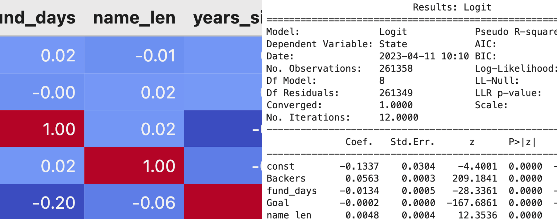
expl.corr().style.background_gradient(cmap='coolwarm', axis=None).set_precision(2)
| Goal | Backers | fund_days | name_len | years_since | |
|---|---|---|---|---|---|
| Goal | 1.00 | 0.01 | 0.02 | -0.01 | 0.02 |
| Backers | 0.01 | 1.00 | -0.00 | 0.02 | 0.03 |
| fund_days | 0.02 | -0.00 | 1.00 | 0.02 | -0.20 |
| name_len | -0.01 | 0.02 | 0.02 | 1.00 | -0.06 |
| years_since | 0.02 | 0.03 | -0.20 | -0.06 | 1.00 |
Figure 1. Plot of correlation matrix for explanatory variables listed in Table 1. Values indicate correlation coefficients between variables.
In Table 1 and Figure 1 above, we can see that there is very weak correlation between our explanatory variables. We do see a correlation coefficient of $r=-0.197$ between the variables years_since and fund_days. However, this value is well below the $r=0.7$ threshold that is commonly used as a rule of thumb for determining if colinearity is present between two variables. Thus, we will keep both of these variables for the moment and move on to our assessment of multicolinearity below.
Above, we determined that there is no evidence of colinearity between our numeric explanatory variables. However, multicolinearity can still occur even if no pair of variables is highly correlated. Thus, we should test for multicolinearity between our numeric explanatory variables by examining the variance inflation factor (VIF) for each variable.
We can test for multicolinearity with the variance_inflation_factor() function from the statsmodels module, which returns a VIF value for each numeric explanatory variable:
vif = [variance_inflation_factor(expl.values, i) for i in range(len(expl.columns))]
print(pd.DataFrame(vif, expl.columns, columns=["VIF"]))
                  VIF
Goal         1.002171
Backers      1.015185
fund_days    4.494515
name_len     4.357918
years_since  4.089828
The statsmodels documentation suggests that VIF values greater than five indicate multicolinearity. As seen above, each of our VIF values is below five, suggesting that multicolinearity is not present among our explanatory variables.
According to Bujang et al. (2018), studies that utilize logistic regression should have a minimum sample size ($n$) of 500, or a sample size where $n = 100 + 50(i)$ (where $i$ is equivalent to the number of explanatory variables in the model). As described in the first section of this analysis, we have nine explanatory variables of interest in our dataset. So, using the rule of thumb above, we would need a sample size of $n = 100 + 50(9) = 550$ observations.
Let's take a look at the number of observations in our dataset below:
print(data.shape[0])
261358
We have 261,358 unique observations in our sample. Thus, it appears that we have a sample size that is sufficient for use in a logistic regression model.
We have verified that our data meets the basic requirements for logistic regression, and are now ready to actually fit our logistic regression model!
First, we'll break up our response and explanatory variables into separate dataframes:
#Split dataset into 'features' and 'target variable'
feature_cols = ['Backers', 'fund_days', 'Goal', 'name_len', 's_spring', 's_summer', 's_fall', 'years_since']
x = data[feature_cols]
y = data['State']
Note that we omit the s_winter column from our explanatory variables. This will allow us to interpret model coefficients for s_spring, s_summer, and s_fall relative to that for s_winter.
Next, we'll create a logistic regression model using the Logit() function from the statsmodels module and display the results below:
#Add an intercept (i.e., a column of 1's) to x
x = sm.add_constant(x)

#Describe the model (statsmodels.discrete.discrete_model.Logit)
model = sm.Logit(endog=y, exog=x, missing='none')

#Fit the model
result = model.fit()

#Print model results (beta coefficients, p-values, and confidence intervals)
res = result.summary2()
print(res)
Optimization terminated successfully.
         Current function value: 0.325689
         Iterations 12
                          Results: Logit
==================================================================
Model:              Logit            Pseudo R-squared: 0.521
Dependent Variable: State            AIC:              170260.9627
Date:               2023-04-11 14:08 BIC:              170355.2255
No. Observations:   261358           Log-Likelihood:   -85121.
Df Model:           8                LL-Null:          -1.7765e+05
Df Residuals:       261349           LLR p-value:      0.0000
Converged:          1.0000           Scale:            1.0000
No. Iterations:     12.0000
-------------------------------------------------------------------
              Coef.   Std.Err.      z      P>|z|    [0.025   0.975]
-------------------------------------------------------------------
const        -0.1337    0.0304    -4.4001  0.0000  -0.1933  -0.0741
Backers       0.0563    0.0003   209.1841  0.0000   0.0558   0.0568
fund_days    -0.0134    0.0005   -28.3361  0.0000  -0.0143  -0.0125
Goal         -0.0002    0.0000  -167.6861  0.0000  -0.0002  -0.0002
name_len      0.0048    0.0004    12.3536  0.0000   0.0040   0.0055
s_spring      0.0301    0.0175     1.7184  0.0857  -0.0042   0.0644
s_summer     -0.1262    0.0175    -7.2137  0.0000  -0.1605  -0.0919
s_fall       -0.0431    0.0179    -2.4067  0.0161  -0.0782  -0.0080
years_since  -0.0889    0.0031   -28.7278  0.0000  -0.0949  -0.0828
==================================================================
The final step in this process is to back-transform coefficients and confidence intervals:
#Define coefficient table from results summary
coef_table = res.tables[1]

#Correct column names
cols = coef_table.columns
coef_table = coef_table[1:]
coef_table.columns = cols.astype(str).str.strip(" ")

#Add back-transformed columns for beta coefficients and confidence intervals
coef_table["OR"] = np.exp(coef_table["Coef."].astype(float))
coef_table["CI_Lower"] = np.exp(coef_table["[0.025"].astype(float))
coef_table["CI_Higher"] = np.exp(coef_table["0.975]"].astype(float))

#Display table
coef_table = pd.concat([coef_table.iloc[:,-3:], coef_table.iloc[:,3]], axis=1)
coef_table
| OR | CI_Lower | CI_Higher | P>|z| | |
|---|---|---|---|---|
| Backers | 1.057927 | 1.057369 | 1.058485 | 0.000000e+00 |
| fund_days | 0.986670 | 0.985755 | 0.987587 | 1.240029e-176 |
| Goal | 0.999760 | 0.999757 | 0.999763 | 0.000000e+00 |
| name_len | 1.004784 | 1.004024 | 1.005546 | 4.657128e-35 |
| s_spring | 1.030556 | 0.995777 | 1.066550 | 8.572709e-02 |
| s_summer | 0.881415 | 0.851699 | 0.912168 | 5.444942e-13 |
| s_fall | 0.957812 | 0.924775 | 0.992031 | 1.609632e-02 |
| years_since | 0.914976 | 0.909446 | 0.920540 | 1.717033e-181 |
Table 2. Odds ratios, back-transformed confidence intervals, and p-values for each explanatory variable in our logistic regression model.
In Table 2 above, we have odds ratios as well as lower and upper bounds of our confidence intervals and associated p-values in the OR, CI_Lower, CI_Higher, and P>|z| columns, respectively. We are now ready to interpret our model.
Using the information contained in Table 2, we can make the following determinations:
Campaigns with more backers have higher odds of success. For every 10 backers that support a campaign, the odds of that campaign's success increase by 75.61% (p < 0.00; 95% CI [74.69%, 76.54%]).
Campaigns with higher fundraising goals have lower odds of success. For every $1,000 USD increase in a campaign's fundraising goal, the odds of that campaign's success decrease by 21.34% (p = 0.00; 95% CI [-21.57%, -21.10%]).
Longer campaign duration is associated with lower odds of success. For every week in a campaign's fundraising period, the odds of that campaign's success decrease by 8.97% (p < 0.00; 95% CI [-9.56%,-8.37%]).
Campaigns launched in winter have higher odds of success than campaigns launched in summer or fall. The odds of success are 11.86% lower for campaigns launched during summer instead of winter (p < 0.00; 95% CI [-14.83%, -8.78%]), whereas the odds of success are 4.22% lower for campaigns launched during fall instead of winter (p = 0.02; 95% CI [-7.52%, -0.80%]). The odds of success for campaigns launched in spring were not significantly different from those for campaigns launched in winter.
Newer campaigns have lower odds of success than those that were launched closer to when Kickstarter was founded. For every year since 2009 - the year in which Kickstarter was initially launched - the odds of campaign success decrease by 8.50% (p < 0.00; 95% CI [-9.06%, -7.95%]).
The effect of campaign name length on odds of success is significant but neglible. For each character in a campaign's name, the odds of success increase by 0.48% (p < 0.00; 95% CI [0.40%, 0.55%]). This effect size is substantially smaller than those of other explanatory variables in our model.
So, according to our model, we see that Kickstarter campaigns with a high number of backers, low fundraising goals, and short fundraising periods have the highest odds of success. Additionally, campaigns that are launched in winter months may have higher odds of success than those launched in other seasons (i.e., summer and fall). These factors appear to be particularly important in predicting campaign success, whereas other factors - such as campaign name length - appear to be less important.
Our results seem like common sense - i.e., that popular campaigns with a lot of supporters and relatively modest fundraising goals are more likely to succeed than unpopular campaigns with high fundraising goals. Regardless, our results could be useful to individuals who are planning to launch Kickstarter campaigns and want to maximize their odds of success!
To explore how this data was cleaned prior to analysis, visit the link below:
View Data Exploration/Cleaning